Matrix Performance

I've recently released version 1.1.1 of Thorwin Math (a Java math library). In this post I will discuss some performance aspects for basic matrix operations. Before reading this post, make sure you've read the previous post about the design of the matrix implementation.

In this post I've included some comparisons with the EJML library. I've included these as EJML provides the best performing single-threaded, non-native matrix implementation for small to medium sized matrices I know of. Note that I've used the simplest way of performing the operations in EJML, as I am attempting to highlight design/performance aspects of Thorwin Math matrices, not making a balanced performance comparison.

Matrix Operations Performance

Lets first take a look at the performance characteristics of the addition of two matrices. First, we take a look at small matrices. The following graph shows the performance for A_(d,d) + B_(d,d) and A_(d,d) + B^'_(d,d).

As very small matrices (up to and including 5x5) are generated and do not use arrays, adding them is faster than EJML. Having no branches, better data locality, opportunities for compiler optimization, and lack of array initialization results in better performance of these very small matrices.

At dimensions in access of 5x5 this advantage is lost. At this point Thorwin Math will use a regular packaged array based implementation, which results in performance that is comparable to EJML.

Adding a transposed matrix for very small (up to and including 5x5) matrices performs really well, as transposing is completely generated and consists of creating a new instance of an object.

At dimensions in access of 5x5, the packed array implementation is used. As the packed array implementation supports both row-major and column-major, it can perform the addition and transposing in a single pass. This results in better performance than performing a transpose on the data, followed by an addition.

The following chart shows the performance of the addition for larger matrix dimensions.

For larger matrices, the addition is implemented using multiple threads. There is a speed-up compared to the single-threaded EJML baseline. It does not, however, scale up to the number of cores (in this case 4), as it bound by memory speed.

The following charts shows multiplication of (square) matrices at various dimensions. We start with small matrix dimensions.

The generated matrices up to and including 5x5 show a definite performance advantage over the packed array implementation. From dimensions of 6 and up the advantage is gone and the performance is on-par with EJML. The Thorwin Math implementation shows a slight performance advantage. I think this is just due to the fact that Thorwin Math operates directly on the packed array, where EJML's SimpleMatrix uses an extra layer of indirection.

The followng chart shows medium to large matrices. This chart includes the performance of Thorwin Math using the accelerator (Thorwin Math Accelerator).



Thorwin Math and EJML stay on-par up to the moment Thorwin Math switches to the block matrix implementation. From this point Thorwin Math starts to use multiple threads. From dimensions around 150 the performance seems to wobble somewhat. This is likely because of the block size or 32x32. As matrix dimensions are not multiples of 32, padding is added. This padding takes part in the multiplication, slowing down when there is relatively large amounts of padding. This is the case around dimensions of 150.  At 160 (5*32), speed is optimal again. At higher dimensions, the padding is relatively insignificant, so the wobble is not visible.

What is very clear in this chart is that native, optimized code is a lot faster than the regular Java code.

This last chart shows multiplication performance for larger matrices. This shows that even at these dimensions, native optimized code outperforms the Java code by a factor of about 2, which is a lot less than at dimensions below 1000.

At dimension of 5000x5000 the multi-threaded Thorwin Math multiplication seems to be almost 4 times as fast as the single-threaded EJML baseline. It seems the algorithm scales well for the number of cores in use.

 

Matrix Design

I have recently released version 1.1.0 of Thorwin Math. In this post I will explain some aspects of the design of the matrices.

API Design

The API of matrices is object-oriented and relatively small. It has been designed to be easy to use and still perform well. The Matrix API is quite similar to JAMA, although there are some important differences.

• Matrix is an interface definition, not a base class.
  
• Matrix instances are immutable. 
• Parallel algorithms are used to utilize modern CPU architectures.
• API is compatible with Java Operator Overloading.
• Matrix uses heterogeneous data storage implementations.
• Designed for Java 8
• Optional native acceleration

A small number of fixed-dimension matrices are available as classes. These include 2D and 3D affine matrices and rotation matrices. These special purpose matrices are provided as they are often required in 2D/3D applications and require optimal performance and type safety.

Having a Matrix interface instead of an abstract base class allows for more design options when integrating with other (matrix) libraries. It also may take advantage of future Java features such as value-types, which currently seem to exclude class hierarchies, but allow interfaces.

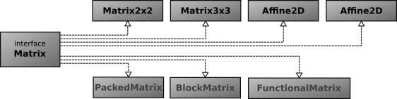
Matrix interface, public and package private implementations

General Matrix Implementation

General matrices are constructed using static methods on the Matrix interface. These methods will return a matrix implementation suitable for the specified data. The matrices returned by these methods are generally not part of the public API, but package private classes. The type of the returned matrix is chosen based on the specified dimensions of the matrix. There are three categories of matrices.

Small Matrices

Small matrices are matrices with dimensions up to 5x5. Small matrices have generated classes for each possible dimension (Matrix1x1, Matrix1x2, etc). At this scale there are some significant advantages of having generated classes:

• Elements are stored as individual instance variables instead of in arrays. 
• No dereferences required for accessing element values.
• No bounds checking on indices.
• Better locality for data.
• Less data used.
• Better compiler optimizations available for (final) instance variables.
• Operations are implemented in generated code
• No loops
• No index calculations performed as all elements are available as fields.
• No dimension checks required for generated classes as type system already provides the guarantees.
• Algorithm optimizations possible when dimensions are known in advance.

The limiting factor for using generated classes for matrices is the number of elements in the matrix, as these need to be passed in the constructor. The number of arguments allowed in a constructor is limited to 256. The practical limit, however, is lower than that because of the sheer number of generated classes and performance characteristics.
Currently having all matrices up to 5x5 generated seems to be a good balance as this includes some matrix dimensions that are very common indeed. The matrix implementations Matrix2x2 and Matrix3x3 are examples of such often used matrices. These matrices are part of the public API, in contrast to the other generated matrices.

Medium Matrices

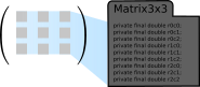
Medium sized matrices are matrices with dimensions up to about 100x100. Medium sides matrices are implemented using a PackedMatrix implementation. This implementation stores element values in a packed array.
The element values are stored in either a row-major (as shown in the illustration) or column-major packed array. This means that transposing a matrix does not involve any operations on the stored elements, just a different ordering state. Other operations can generally efficiently operate on both row-orderings, which means that transposing a matrix does not involve much (or any) overhead.
Using a packed array for data storage is limited mostly by data locality. For instance in a row-major packed array, elements in a single column are not stored together in memory.

Large Matrices

Large matrices are matrices with dimensions in excess of about 100x100. Large matrices are implemented using a BlockMatrix. This implementation stores matrix elements in 32x32 sub-matrices. This provides much better data locality than using a packed array.
Operations such as addition, subtraction, multiplication and scaling are implemented using parallel algorithms, speeding up the execution on multi-core and multi-processor systems.
If a sub-matrix is known to only contain zero values, it will not store this data. Basic operations will take advantage of this knowledge and perform considerably better.
There is currently no specific support for band or sparse matrices. These matrices may, however, take some advantage of the empty sub-matrix optimizations.

Functional Matrix

A special type of matrix is provided to allow functional style definition of a matrix. A single lambda function defines the element data of the matrix, which is a very flexible way of constructing a matrix. Basic operations will result in new functional matrices, providing lazy evaluation without intermediate data storage. For example, an 100x100 identity matrix can be created using the following instruction:

Matrix.function(100,100, (row,column)-> row == column ? 1 : 0);

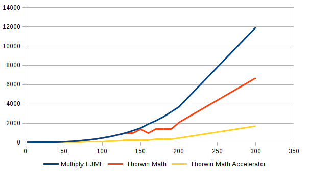
Low-level API and Native Accelerators

The low-level API provides support for some matrix operations. It can be used to optimize performance critical algorithms that can benefit from this low-level code. The low-level API operates on packed byte arrays.

The low-level API has been designed to be replaced by a native implementation. Using a native accelerator, some operations (i.e. matrix multiplication) can be accelerated considerably. As the low-level API is used by Matrix implementations, using an native accelerator will also boost their performance.

A native accelerator has been implemented for Intel x64 processors using OpenBLAS.

MATLAB/Octave

Matrices can be constructed from a text string. The format is similar and compatible with the format used in MATLAB/Octave. This means you can construct a matrix like this:

Matrix.valueOf("1,2;3,4");

The string representation of a matrix is similar to MATLAB/Octave and can also be used to create a matrix from a text string. This means that matrix input and output can be copied from MATLAB/Octave to Java code.

This is particularly useful when porting code and creating unit tests.

Links

• Thorwin Math
• Java Matrix Package (JAMA) 
• Java Operator Overloading (Java-OO)

Porting Matrix and Vector Algorithms using Java-OO and CFR

Porting algorithms between Java and other languages can be quite cumbersome. Different languages have different features, some of which may be difficult to port. When dealing with vectors and matrices, in my experience important differences in languages are:

• Language support for matrices/vectors
• Operator-overloading
• Mutable or immutable matrices/vectors
• Zero or one based indices

In this post I will discuss operator-overloading when porting algorithms to Java.
Operator overloading is not a feature supported by the Java language. Java-OO is a project that provides basic operator overloading support to the Java language. In this post I will discuss the use of this software in combination with the Matrix and  Vector classes in the thorwin-math library.

Before you can execute the example, set-up your IDE:

• Download thorwin-math.*.jar and add it as library to your project. This file can be downloaded from thorwin.nl.
• Download and install Java-OO for your compiler/IDE of choice. The Java-OO site is located here. It may be a good idea to check over the features of Java-OO before continuing.

Constructors

Ok, lets take a look at constructors first. As thorwin-math is designed to be used with Java-OO, the Matrix and Vector classes provide static valueOf methods for constructing instances. Using Java-OO, these constructors are automatically found and used when assigning arrays or strings. Take a look at the following code:

double[] vectorArray = {1, 2, 3};
Vector v1 = vectorArray;
Vector v2 = "4 5 6";

double[][] matrixArray = {{1, 2, 3}, {4, 5, 6}};
Matrix m1 = matrixArray;
Matrix m2 = "1 2; 3 4; 5 6";

The first line contains the conversion of an array of doubles to a Vector. Although the valueOf method itself is very clear, this automatic conversion is quite nice when mixing the Vector class with existing code that uses arrays, when porting C code to Java for instance.

The conversion from a string is not the fastest way to construct a vector, but it is very clear and consise. When writing unit tests this notation is very nice, as I can cut and paste values between MATLAB and Java.

The conversion for the Matrix class are very similar. Again, the main use here is conversion of 2D arrays to matrices and interoperability with MATLAB.

Operators

The following code shows some examples of vector and matrix calculations, when using Java-OO.

Vector v3 = v1 + v2;
Vector v4 = v1 - v2;
Vector v5 = -v1;

Matrix m3 = m1 + m1;
Matrix m4 = m1 - m1;
Matrix m5 = -m1;
Matrix m6 = m1 * m2;
Vector v6 = m1 * v1;

double dot = v1 * v2;

This is all pretty much what you expect when using operator overloading. Java-OO really helps to implement algorithms from pseudo-code or porting from languages such as C#, C++ or MATLAB.

Element Access

Java-OO even provides array-like element access, which is really helpful to port code that uses arrays for vector values (C) or code that also has support for this (C++).

double element = v1[2];

Array-like assignment is also possible in Java-OO, but not with thorwin-math vectors, as these are immutable.

Note that Java code uses zero based indices. Special care must be taken when porting code that is has 1-based indices (MATLAB).

Removing Java-OO

Java-OO is very helpful for creating and maintaining math code.  Current support for compilers and integrated development environments is very good. There may still, however, be a good reason for not wanting a build dependency to Java-OO.

This is where a good Java decompiler is a valuable tool. I currently use CFR, which is a nice decompiler with Java 8 support. You can find it here.

Take, for example, the following piece of Java code that uses Java-OO:

Matrix m = (a + b) * (c - d);

This code can be compiled as part of some Java class. The resulting class file can be decompiled to regular Java code using CFR. The code snippet above is decompiled to:

Matrix m = a.add(b).multiply(c.subtract(d));

We end up with regular Java code.

Trend Curve/Line in JavaFX Chart

JavaFX provides some nice components for displaying various kinds of charts. Displaying sample data in a line or scatter chart is quite easy. Interpreting sample data to display trends is more challenging. In this post I will show how to create a chart showing sample data and and a trend curve.

The following illustration shows the end result. It shows both the samples in red and an orange trend curve.

The Java Code

To create the trend curve, I've used a polynomial fitting algorithm to calculate the best fitting polynomial coefficients. The sample code uses the polyfit and polynomial methods from thorwin.math.Math, which can be downloaded here.

import javafx.application.Application;
import javafx.scene.Scene;
import javafx.scene.chart.LineChart;
import javafx.scene.chart.NumberAxis;
import javafx.scene.chart.XYChart;
import javafx.stage.Stage;

import static thorwin.math.Math.polyfit;
import static thorwin.math.Math.polynomial;

public class Demo extends Application {

    @Override
    public void start(Stage primaryStage) throws Exception{

        // stup the chart
        XYChart.Series<Number,Number> series1 = new XYChart.Series<>();
        XYChart.Series<Number,Number> series2 = new XYChart.Series<>();

        NumberAxis xAxis = new NumberAxis();
        NumberAxis yAxis = new NumberAxis();

        LineChart<Number,Number> chart = 
            new LineChart<Number, Number>(xAxis, yAxis);

        chart.getData().add(series1);
        chart.getData().add(series2);
        chart.getStylesheets().add(Demo.class.getResource("style.css")
             .toExternalForm());

        // setup chart series
        double[] xs = {0.0, 1.0, 2.0, 3.0, 4.0, 5.0};
        double[] ys = {0.5, 1.3, 2.4, 5.6, 8.8, 9.1};

        for (int i = 0; i < xs.length; i++) {
            series1.getData().add(new XYChart.Data<>(xs[i], ys[i]));
        }

        // calculate the polynomial coefficients and calculate trend points
        double[] coefficients = polyfit(xs, ys, 2);

        for (double x = 0; x <= 5.0; x += 0.05) {
            double y = polynomial(x, coefficients);
            series2.getData().add(new XYChart.Data<>(x,y));
        }

        // setup scene and stage
        Scene scene = new Scene( chart );

        primaryStage.setScene(scene);
        primaryStage.sizeToScene();
        primaryStage.show();
    }


    public static void main(String[] args) {
        launch(Demo.class, args);
    }
}

The polyfit method calculates the polynomial coefficients the the polynomial that fits the sample points best. I've chosen a 2nd order polynomial, which is a curve. If you want a trend line instead of a curve, use a first order polynomial. Higher order polynomials are also possible, just experiment a little.

Stylesheet

The chart we're creating looks like a combination of a scatter chart and a line chart. We could use two charts and try to combine them into one, but applying some styling to the line chart seems to work as well.

The code refers to a file 'style.css', which contains the following stylesheet:

.default-color0.chart-series-line {
    -fx-stroke: transparent;
}

.default-color1.chart-line-symbol {
    -fx-background-color: transparent;
}

This stylesheet will hide lines of the sample data (first data series). It also hides the sample points of the trend curve (second data series).